Avoid the heatwave!

The past week, San Diego experienced an abysmal heatwave. It not only terrorized the day, but it also haunted my good night’s sleep - I would wake up in the middle of the night with my neck wet from sweat.

This conundrum motivated me to make a path planning algorithm that avoids the sunlight and “seeks” the shade (a penalty if you are in the sun).

In explaining this, I'll start with the algorithm, and then move to the more nitty-gritty maths (it's still simple! just will seem a bit overwhelming if I put it in the beginning). Also, if you want to try the algorithm, scroll to the bottom!

1.Modelling the shadow

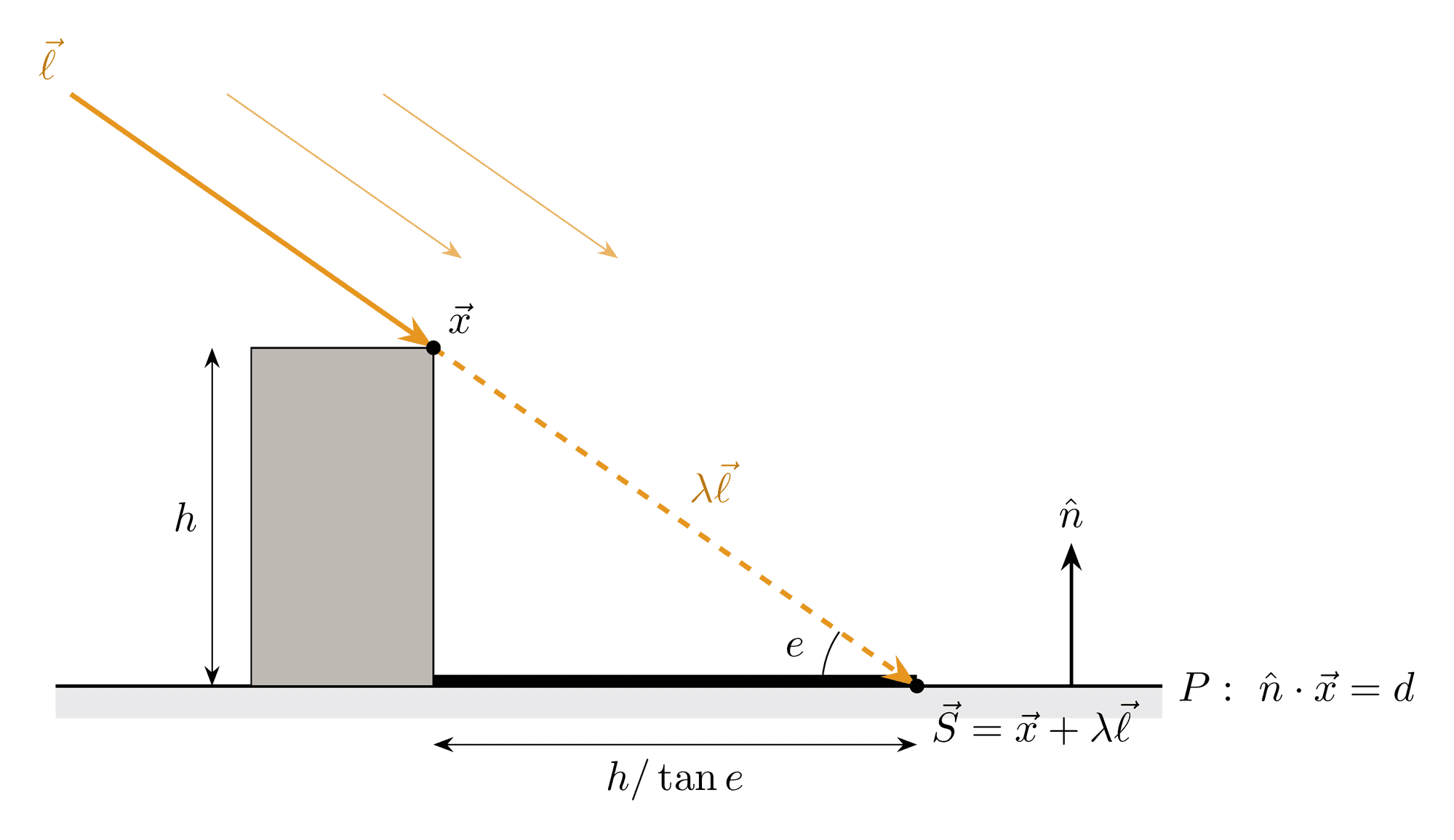
Let’s start by thinking about shadows, so we get a gist of what we’re working with. Frankly, this section won’t be helpful until we have figured out the algorithm.

Here, we’ll use the parallel light rays model. Assume the sun emits parallel rays . If we have a plane in Hessian form, , then the shadow of a point is simply where the ray through along lands on the plane. That ray is , so its intersection with is

2.The modified A* algorithm

Since we still want to find the shortest path, A* is our best friend. To recap, here’s how the A* algorithm works:

import heapq

def a_star(start, goal, neighbors, d, h):
    open_set = [(h(start), start)]  # min-heap of (f, node)
    came_from = {}
    g_score = {start: 0}

    while open_set:
        _, current = heapq.heappop(open_set)  # lowest f first
        if current == goal:
            path = [current]
            while current in came_from:
                current = came_from[current]
                path.append(current)
            return path[::-1]

        for neighbor in neighbors(current):
            tentative_g = g_score[current] + d(current, neighbor)
            if tentative_g < g_score.get(neighbor, float("inf")):
                came_from[neighbor] = current
                g_score[neighbor] = tentative_g
                heapq.heappush(open_set, (tentative_g + h(neighbor), neighbor))

    return None  # no path

In simple words, we minimize at every step:

where is the cost of the path we have gone through, and is the heuristic we use to estimate the cost still left to reach the goal - so when the cost is just distance, people typically use the Euclidean or the Manhattan distance.

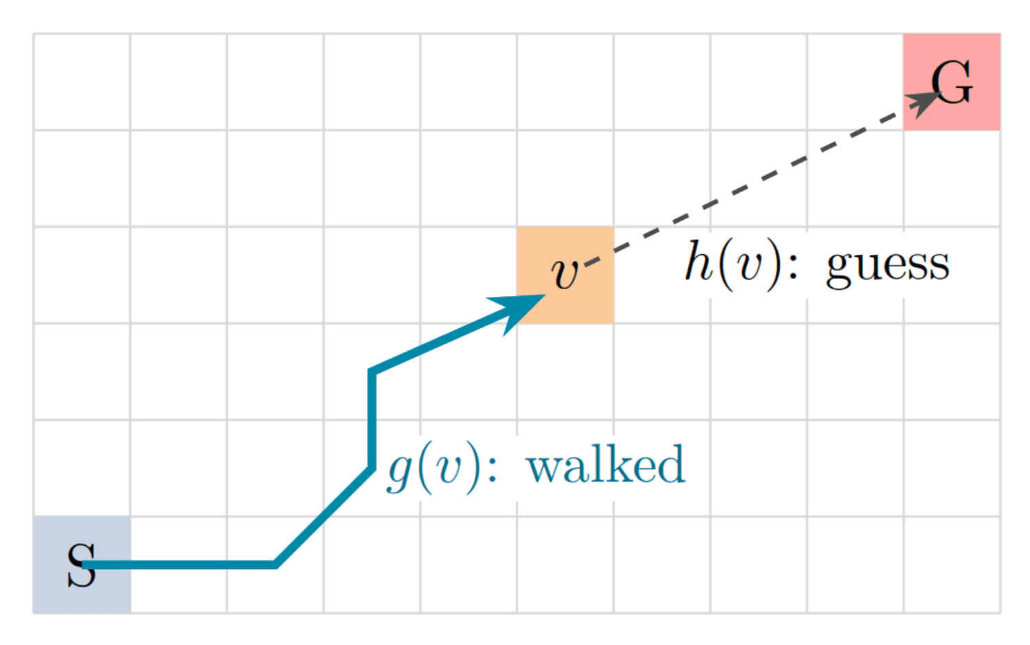
However, picking the minimal is just a way of deciding where to explore next. Once we pick that cell, we look at each of its neighbors and compute a new for it: the cost of reaching that neighbor through the current cell. If this new is lower than the the neighbor already had, we’ve found a cheaper route to it, so we update its and remember the current cell as its parent. Otherwise we leave it alone. When we finally reach the goal, we follow these parents back to recover the path.

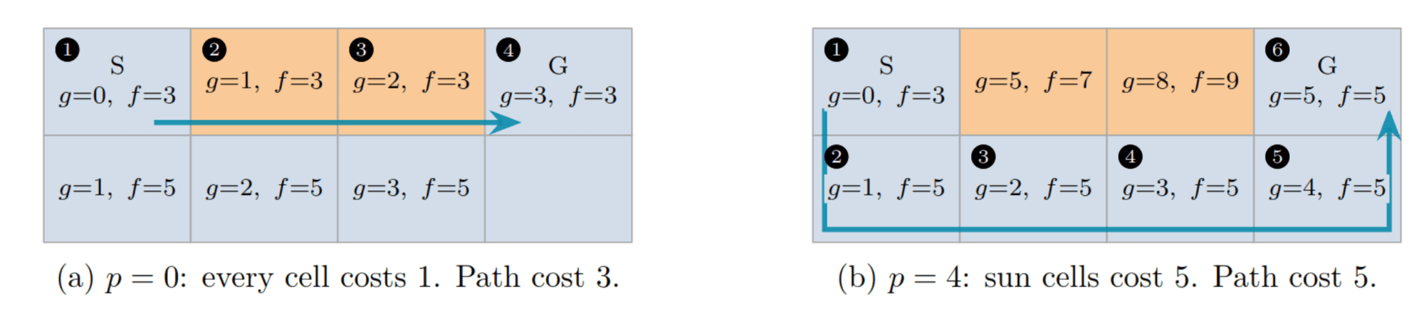
We will add a penalty to (the path cost) so that heat gets considered. Assume is the extra cost, so:

where is our path cost for this modified algorithm and is the usual path cost, which in our case means the distance we have walked so far. For the heuristic, we’ll use the typical Euclidean distance, nothing fancy:

3.The extra cost function

Intuitively, if the sun is directly on top of us, it’s far brighter and hotter. If its elevation is lower, it’s less intense. This is a simple explanation for Lambert’s cosine law - the equation we’ll use for the penalty:

where is the sun’s irradiance and is the irradiance “felt” by the surface. Here is measured from the surface normal, not the ground. For flat ground with the sun at elevation , , so

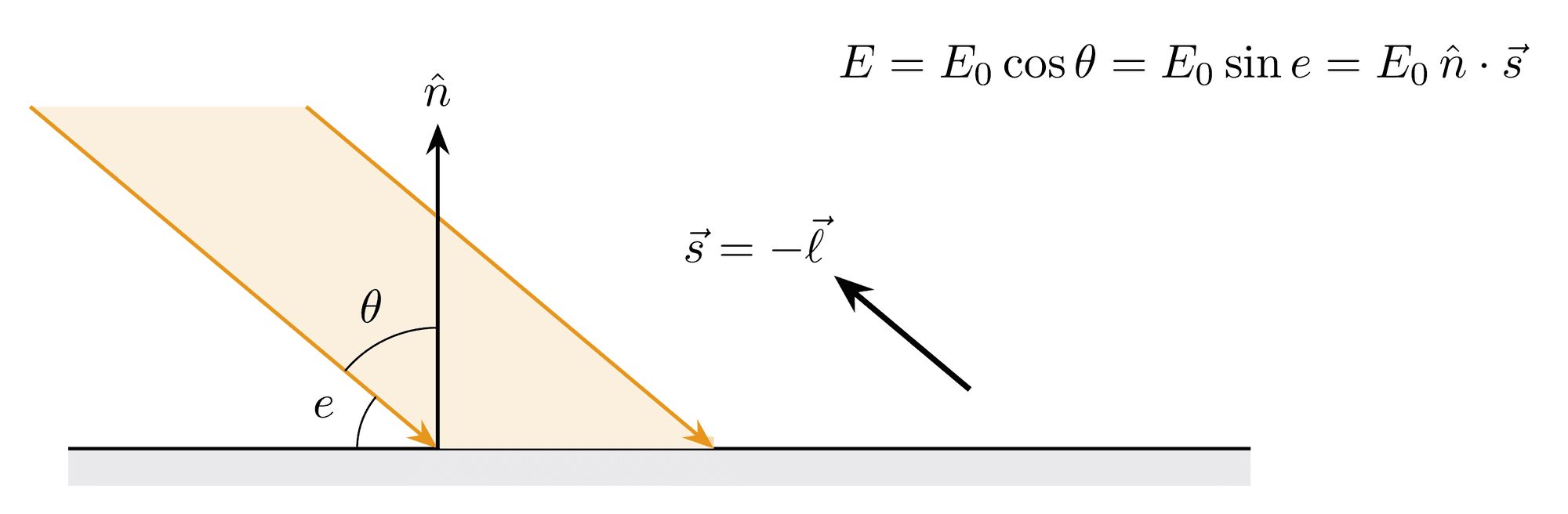
where points toward the sun. Combining this with the intensity of light that we'll further explain in section 5:

Shaded cells have regardless of the sun; sunny cells get hotter as the sun climbs. Finally, the extra cost per metre of a cell is

where is the heat penalty, a single number (set by a slider) that is the same for every cell. Summed along a path, the total cost becomes

i.e. the distance walked plus times the “metres of sun”. So acts as an exchange rate: A* will walk up to extra metres to avoid one metre of full sun.

Here’s the search itself, where each cell’s cost is :

import heapq
import math

MOVES = [(dr, dc, math.hypot(dr, dc)) for dr in (-1, 0, 1) for dc in (-1, 0, 1) if dr or dc]


def astar(cost, blocked, start, goal):
    rows, cols = cost.shape
    cost, blocked = cost.tolist(), blocked.tolist()
    g = [[math.inf] * cols for _ in range(rows)]
    parent = {}
    g[start[0]][start[1]] = 0.0
    frontier = [(math.dist(start, goal), 0.0, start)]
    while frontier:
        _, g_cur, cur = heapq.heappop(frontier)
        if cur == goal:
            path = [cur]
            while cur in parent:
                cur = parent[cur]
                path.append(cur)
            return path[::-1]
        r, c = cur
        if g_cur > g[r][c]:
            continue
        for dr, dc, step in MOVES:
            nr, nc = r + dr, c + dc
            if not (0 <= nr < rows and 0 <= nc < cols) or blocked[nr][nc]:
                continue
            if dr and dc and (blocked[nr][c] or blocked[r][nc]):
                continue
            g_new = g_cur + step * 0.5 * (cost[r][c] + cost[nr][nc])
            if g_new < g[nr][nc]:
                g[nr][nc] = g_new
                parent[(nr, nc)] = cur
                heapq.heappush(frontier, (g_new + math.dist((nr, nc), goal), g_new, (nr, nc)))
    return None

Awesome, so that’s our avoid-the-heatwave A* algorithm. Nevertheless, we need to build the world to see how the algorithm works and define the equation for heat. For the world, ideally we want to implement it with SDFs in mind for versatility. I’ll explain SDFs and shadow tracing, but will skip baking and primitives.

4.The world as signed distance functions

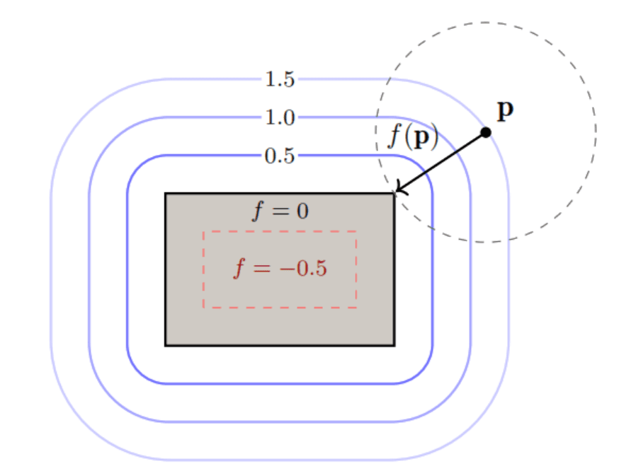
An SDF gives, for any point , the distance to the nearest surface, with a sign:

The key property: a ball of radius around contains no solid. Additionally, shapes are combined with simple operations, e.g. union is and subtraction is , so a whole city is just one function.

5.Shadow tracing

Okay, so back in section 1, we asked: where does the shadow of a point land?

That works for solid objects, but it gets kinda messy when we work with hollow objects. So we flip the question: from a ground point , does a ray toward the sun hit anything?

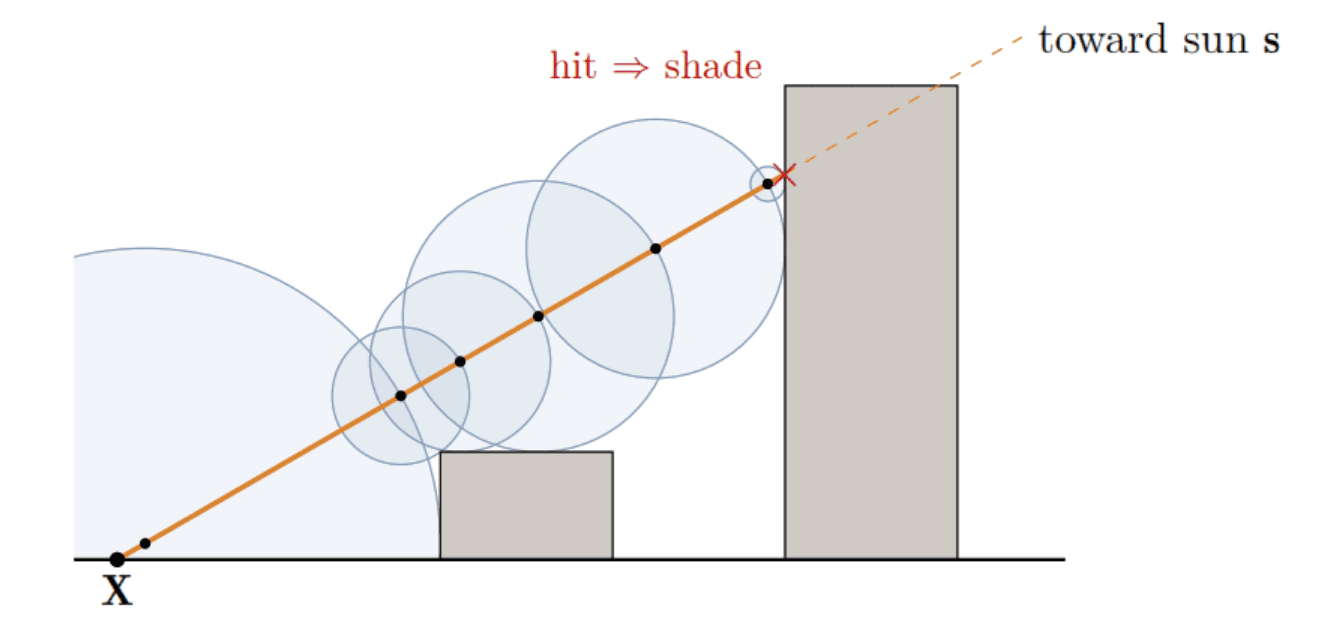
Basically, if the ray hits something on the way to the sun, we’re in the shade. Same shadow, just asked backwards. So how do we check if the ray hits something? Sphere tracing! Imagine walking from toward the sun along

where is how far we’ve walked (in metres) and is where we are. At every step, we ask the SDF “how far is the closest wall?” and just walk that far:

where is the step number. This is safe because nothing is inside that ball (section 4), so we can never walk through a wall. Close to a wall the steps get tiny, and once is basically zero () we’ve hit it, so is in shade ( is the "close enough to touching" threshold). If we walk out of the world without hitting anything, is in full sun.

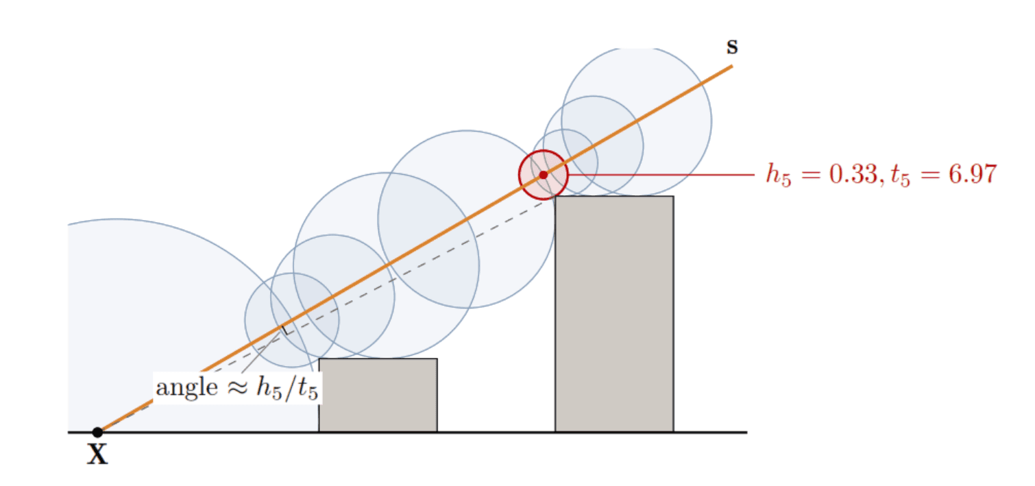
Now, in real life, shadow edges are kind of blurry, meaning that we need to consider rays that “almost” hit something. At each step, is how close we pass to a wall, and is how far we are from . Seen from , that near-miss looks like an angle of about . The closest near-miss decides how much light gets through:

where controls how sharp the edge is - a variable in our code. Clamp just keeps the answer between 0 (full shade) and 1 (full sun). (Here is just a distance, not the A* heuristic.) A huge gives back the sharp shadow from section 1. The real sun would be around , but I use so the planner stays a bit away from shadow edges.

And this light is exactly what we plug into in section 3. So the full pipeline is: shadow tracing → heat → cost → A*.

And that’s it! Here’s the full pipeline of avoid the heatwave:

And here it is running. This is the actual Python - world.py, sdf.py, render.py and astar.py - running in your browser with Pyodide. Tap to place the start or goal (right-click places the goal), drag the sun around, or let it move: